Organizing and simplifying code using functions
How to reuse your code… Use functions!
- Use a piece of code more than once? Create a function!
- Have a bit of code that is complex or fairly complicated? Create functions!
Why use functions:
- Makes your code more readable
- Let’s you reuse complex or repetitive code easily
- Uses the DRY principle: Don’t Repeat Yourself
What is a function:
- An encapsulated piece of code
- Takes an input or set of inputs, and outputs a single object
- R is a functinal programming language: Every action is a function in R
- ie.
mean(),plot(),[,<-, etc.
- ie.
Creating a function
- Each function is composed of at least three to four parts:
- Assignment
<-as an object (optional) - The
functioncall and if needed the arguments (aka options/settings) - The code within the function
- Final object/data to output (the
return)
- Assignment
- Make your code more readable, name your function descriptively:
scatter_plotnot e.g.someplotextract_pvaluenot e.g.porvalue
- Be descriptive with the code in the function too
A function looks like:
# Anonymous function
function(arg1, arg2) {
    #...code content and action...
    return(output)
}

# Named function
function_name <- function(arg1, arg2) {
    #...code content and action...
    return(output)
}
A very simple example:
Add <- function(value1, value2) {
    output <- value1 + value2
    return(output)
}

Add(1, 2) # should be
#> [1] 3Document your functions
Use Ctrl-Shift-Alt-R with cursor in function when using RStudio (only used in
.R files, not .Rmd files)
Should look like:
#' Informative title
#'
#' More detailed description.
#'
#' @param value1 explanation
#' @param value2 explanation
#'
#' @return What it outputs
#'
#' @examples
#' Add(1,2)
if else in functions
- Control how your function works using
if else:
if (condition) {
    true condition
} else {
    false condition
}

if (condition) {
    true condition
} else if (another_condition) {
    true condition
} else {
    false condition
}
Using functions from other packages in your function
Sometimes you’ll come across this ::. For instance:
dplyr::select(iris, Sepal.Length)- This tells R to take the function
selectfrom the packagedplyr. - Better to use this style within a function rather than use
library()- Using
library()within a function is bad practice - Let’s you know which commands come from which package
- Better documents your function
- Makes it more readable and transparent
- Using
Code used in session:
# Build up function without `::` to check that it works
library(ggplot2)
gg_scatterplot <- function(data, x, y) {
    scatter_plot <- ggplot(data, aes_string(x, y)) +
        geom_point() +
        theme_bw() +
        theme(panel.border = element_blank(),
              panel.grid = element_blank(),
              axis.line.x = element_line(colour = 'black'),
              axis.line.y = element_line(colour = 'black')
              )
    return(scatter_plot)
}

gg_scatterplot(iris, 'Sepal.Length', 'Sepal.Width')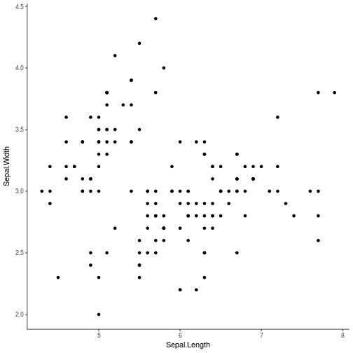
# It works! Now switch to using `::`
gg_scatterplot <- function(data, x, y) {
    scatter_plot <- ggplot2::ggplot(data, ggplot2::aes_string(x, y)) +
        ggplot2::geom_point() +
        ggplot2::theme_bw() +
        ggplot2::theme(panel.border = ggplot2::element_blank(),
              panel.grid = ggplot2::element_blank(),
              axis.line.x = ggplot2::element_line(colour = 'black'),
              axis.line.y = ggplot2::element_line(colour = 'black')
              )
    return(scatter_plot)
}

gg_scatterplot(iris, 'Sepal.Length', 'Sepal.Width')
gg_scatterplot(iris, 'Sepal.Length', 'Petal.Length')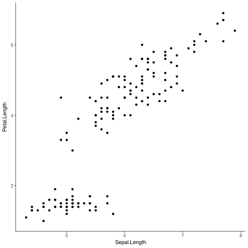
# Using if else conditions
anova_results <- function(data, factor_var, cont_var, tidied = TRUE) {
    Y <- factor(data[[factor_var]])
    x <- as.numeric(data[[cont_var]])
    if (tidied) {
        model <- broom::tidy(aov(x ~ Y))
    } else {
        model <- aov(x ~ Y)
    }
    return(model)
}

anova_results(iris, 'Species', 'Sepal.Length')
#> term df sumsq meansq statistic p.value
#> 1 Y 2 63.21213 31.6060667 119.2645 1.669669e-31
#> 2 Residuals 147 38.95620 0.2650082 NA NAanova_results(iris, 'Species', 'Petal.Length')#> term df sumsq meansq statistic p.value
#> 1 Y 2 437.1028 218.5514000 1180.161 2.856777e-91
#> 2 Residuals 147 27.2226 0.1851878 NA NAanova_results(iris, 'Species', 'Petal.Length', tidied = FALSE)#> Call:
#> aov(formula = x ~ Y)
#>
#> Terms:
#> Y Residuals
#> Sum of Squares 437.1028 27.2226
#> Deg. of Freedom 2 147
#>
#> Residual standard error: 0.4303345
#> Estimated effects may be unbalanced# Tidied version allows you to easily access values for the anova results.
fit <- anova_results(iris, 'Species', 'Petal.Length',
tidied = TRUE)
fit$p.value#> [1] 2.856777e-91 NAfit$sumsq#> [1] 437.1028 27.2226# Compared to...:
fit1 <- anova_results(iris, 'Species', 'Petal.Length',
tidied = FALSE)
fit1$p.value#> NULL# Simple example of using anonymous functions:
processing_data <- function(data, char_var, fun) {
data$NewVar <- fun(data[[char_var]])
return(data)
}
# Use the anonymous function as an argument for the `fun` parameter of the processing_data function.
processing_data(head(iris, 20), 'Species', function(x) {
x <- gsub('setosa', 'Set', x)
x <- as.factor(x)
return(x)
})#> Sepal.Length Sepal.Width Petal.Length Petal.Width Species NewVar
#> 1 5.1 3.5 1.4 0.2 setosa Set
#> 2 4.9 3.0 1.4 0.2 setosa Set
#> 3 4.7 3.2 1.3 0.2 setosa Set
#> 4 4.6 3.1 1.5 0.2 setosa Set
#> 5 5.0 3.6 1.4 0.2 setosa Set
#> 6 5.4 3.9 1.7 0.4 setosa Set
#> 7 4.6 3.4 1.4 0.3 setosa Set
#> 8 5.0 3.4 1.5 0.2 setosa Set
#> 9 4.4 2.9 1.4 0.2 setosa Set
#> 10 4.9 3.1 1.5 0.1 setosa Set
#> 11 5.4 3.7 1.5 0.2 setosa Set
#> 12 4.8 3.4 1.6 0.2 setosa Set
#> 13 4.8 3.0 1.4 0.1 setosa Set
#> 14 4.3 3.0 1.1 0.1 setosa Set
#> 15 5.8 4.0 1.2 0.2 setosa Set
#> 16 5.7 4.4 1.5 0.4 setosa Set
#> 17 5.4 3.9 1.3 0.4 setosa Set
#> 18 5.1 3.5 1.4 0.3 setosa Set
#> 19 5.7 3.8 1.7 0.3 setosa Set
#> 20 5.1 3.8 1.5 0.3 setosa Set
Written on February 1, 2017