Data Wrangling in R
For more detailed notes and explanations, see this webpage. Another great resource for beginners and those learning data analysis and wrangling is the free online book R for Data Science.
Code used during session
library(dplyr)
library(tidyr)
dplyr commands:
- select
- rename
- mutate
- filter
- group_by
- summarise
ds <- read.csv("http://codeasmanuscript.org/states_data.csv")
head(ds)
#> StateName Population Income Illiteracy LifeExp Murder HSGrad Frost
#> 1 Alabama 3615 3624 2.1 69.05 15.1 41.3 20
#> 2 Alaska 365 6315 1.5 69.31 11.3 66.7 152
#> 3 Arizona 2212 4530 1.8 70.55 7.8 58.1 15
#> 4 Arkansas 2110 3378 1.9 70.66 10.1 39.9 65
#> 5 California 21198 5114 1.1 71.71 10.3 62.6 20
#> 6 Colorado 2541 4884 0.7 72.06 6.8 63.9 166
#> Area Region Division Longitude Latitude
#> 1 50708 South East South Central -86.7509 32.5901
#> 2 566432 West Pacific -127.2500 49.2500
#> 3 113417 West Mountain -111.6250 34.2192
#> 4 51945 South West South Central -92.2992 34.7336
#> 5 156361 West Pacific -119.7730 36.5341
#> 6 103766 West Mountain -105.5130 38.6777# %>%
names(ds)#> [1] "StateName" "Population" "Income" "Illiteracy" "LifeExp"
#> [6] "Murder" "HSGrad" "Frost" "Area" "Region"
#> [11] "Division" "Longitude" "Latitude"ds %>%
select(Population, Frost, Area) %>%
filter(Area > 100000)#> Population Frost Area
#> 1 365 152 566432
#> 2 2212 15 113417
#> 3 21198 20 156361
#> 4 2541 166 103766
#> 5 746 155 145587
#> 6 590 188 109889
#> 7 1144 120 121412
#> 8 12237 35 262134#ds[2, ]names(ds)#> [1] "StateName" "Population" "Income" "Illiteracy" "LifeExp"
#> [6] "Murder" "HSGrad" "Frost" "Area" "Region"
#> [11] "Division" "Longitude" "Latitude"ds %>%
mutate(PopPerArea = Population / Area) %>%
select(PopPerArea)#> PopPerArea
#> 1 0.0712905261
#> 2 0.0006443845
#> 3 0.0195032491
#> 4 0.0406198864
#> 5 0.1355708904
#> 6 0.0244877898
#> 7 0.6375976964
#> 8 0.2921291625
#> 9 0.1530227399
#> 10 0.0849103714
#> 11 0.1350972763
#> 12 0.0098334482
#> 13 0.2008502547
#> 14 0.1471867468
#> 15 0.0511431687
#> 16 0.0278772910
#> 17 0.0854224464
#> 18 0.0847095482
#> 19 0.0342173351
#> 20 0.4167424932
#> 21 0.7429082545
#> 22 0.1603569354
#> 23 0.0494520047
#> 24 0.0494967862
#> 25 0.0690919632
#> 26 0.0051240839
#> 27 0.0201874926
#> 28 0.0053690542
#> 29 0.0899523651
#> 30 0.9750033240
#> 31 0.0094224624
#> 32 0.3779139052
#> 33 0.1115004713
#> 34 0.0091955019
#> 35 0.2619890177
#> 36 0.0394725364
#> 37 0.0237461532
#> 38 0.2637548370
#> 39 0.8875119161
#> 40 0.0931679074
#> 41 0.0089658350
#> 42 0.1009727062
#> 43 0.0466822312
#> 44 0.0146535763
#> 45 0.0509334197
#> 46 0.1252136752
#> 47 0.0534625207
#> 48 0.0747403407
#> 49 0.0842574912
#> 50 0.0038681934#names(ds)
ds %>%
select(Population, Income, Frost, Area, LifeExp) %>%
gather(Measure, Value) %>%
group_by(Measure) %>%
summarise(Mean = round(mean(Value), 1),
SD = round(sd(Value), 1),
MeanSD = paste0(Mean, ' (', SD, ')')) %>%
select(-Mean, -SD) %>%
knitr::kable(caption = "Table 1: Basic demographics")| Measure | MeanSD |
|---|---|
| Area | 70735.9 (85327.3) |
| Frost | 104.5 (52) |
| Income | 4435.8 (614.5) |
| LifeExp | 70.9 (1.3) |
| Population | 4246.4 (4464.5) |
ds %>%
    select(Region, Population, Income) %>%
    gather(Measure, Value, -Region) %>%
    group_by(Region, Measure) %>%
    summarise(Mean = round(mean(Value), 1),
              SD = round(sd(Value), 1),
              MeanSD = paste0(Mean, ' (', SD, ')')) %>%
    select(-Mean, -SD) %>%
    spread(Region, MeanSD) %>%
knitr::kable(caption = "Table 2: Characteristics by Region")| Measure | North Central | Northeast | South | West |
|---|---|---|---|---|
| Income | 4611.1 (283.1) | 4570.2 (559.1) | 4011.9 (605.5) | 4702.6 (663.9) |
| Population | 4803 (3702.8) | 5495.1 (6079.6) | 4208.1 (2779.5) | 2915.3 (5578.6) |
#library(tidyverse)
library(ggplot2)
library(tibble)
ds %>%
    select(Population, Income, Frost, Area) %>%
    cor() %>%
    as.data.frame() %>%
    rownames_to_column() %>%
    rename(Var1 = rowname) %>%
    gather(Var2, Correlation, -Var1) %>%
    ggplot(aes(y = Var1, x = Var2)) +
    geom_tile(aes(fill = Correlation))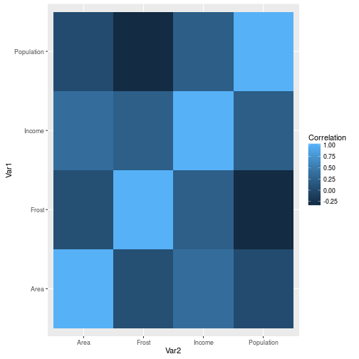
Written on November 9, 2016