Brief introduction to using R and RStudio
The basics: R is a programming language and statistical computing environment. RStudio is an app that allows you to interact with R, but they are created by completely different groups/organizations. Think of R as the backend and RStudio as the frontend.
In the session we went over the layout and use of RStudio, how to send code from
R scrips (.R files), how to use R projects (.Rproj files), and how to
install packages to enhance the abilities of R. Everything in R is an object and
every action is called a function.
Here is some of the code we went over:
# This is a comment

# Look at first 6 rows of the builtin practice dataset called swiss:
head(swiss)
#> Fertility Agriculture Examination Education Catholic
#> Courtelary 80.2 17.0 15 12 9.96
#> Delemont 83.1 45.1 6 9 84.84
#> Franches-Mnt 92.5 39.7 5 5 93.40
#> Moutier 85.8 36.5 12 7 33.77
#> Neuveville 76.9 43.5 17 15 5.16
#> Porrentruy 76.1 35.3 9 7 90.57
#> Infant.Mortality
#> Courtelary 22.2
#> Delemont 22.2
#> Franches-Mnt 20.2
#> Moutier 20.3
#> Neuveville 20.6
#> Porrentruy 26.6# Look at the first 10 rows:
head(swiss, n = 10)#> Fertility Agriculture Examination Education Catholic
#> Courtelary 80.2 17.0 15 12 9.96
#> Delemont 83.1 45.1 6 9 84.84
#> Franches-Mnt 92.5 39.7 5 5 93.40
#> Moutier 85.8 36.5 12 7 33.77
#> Neuveville 76.9 43.5 17 15 5.16
#> Porrentruy 76.1 35.3 9 7 90.57
#> Broye 83.8 70.2 16 7 92.85
#> Glane 92.4 67.8 14 8 97.16
#> Gruyere 82.4 53.3 12 7 97.67
#> Sarine 82.9 45.2 16 13 91.38
#> Infant.Mortality
#> Courtelary 22.2
#> Delemont 22.2
#> Franches-Mnt 20.2
#> Moutier 20.3
#> Neuveville 20.6
#> Porrentruy 26.6
#> Broye 23.6
#> Glane 24.9
#> Gruyere 21.0
#> Sarine 24.4# We can load data by running read.csv. In this case I am importing a dataset
# from my codeasmanuscript website. Assigning the dataset using <- into the ds
# object allows you to use it later in your code.
ds <- read.csv("http://codeasmanuscript.org/states_data.csv")
# Looking at the contents:
head(ds)#> StateName Population Income Illiteracy LifeExp Murder HSGrad Frost
#> 1 Alabama 3615 3624 2.1 69.05 15.1 41.3 20
#> 2 Alaska 365 6315 1.5 69.31 11.3 66.7 152
#> 3 Arizona 2212 4530 1.8 70.55 7.8 58.1 15
#> 4 Arkansas 2110 3378 1.9 70.66 10.1 39.9 65
#> 5 California 21198 5114 1.1 71.71 10.3 62.6 20
#> 6 Colorado 2541 4884 0.7 72.06 6.8 63.9 166
#> Area Region Division Longitude Latitude
#> 1 50708 South East South Central -86.7509 32.5901
#> 2 566432 West Pacific -127.2500 49.2500
#> 3 113417 West Mountain -111.6250 34.2192
#> 4 51945 South West South Central -92.2992 34.7336
#> 5 156361 West Pacific -119.7730 36.5341
#> 6 103766 West Mountain -105.5130 38.6777# Compared with:
ds#> StateName Population Income Illiteracy LifeExp Murder HSGrad Frost
#> 1 Alabama 3615 3624 2.1 69.05 15.1 41.3 20
#> 2 Alaska 365 6315 1.5 69.31 11.3 66.7 152
#> 3 Arizona 2212 4530 1.8 70.55 7.8 58.1 15
#> 4 Arkansas 2110 3378 1.9 70.66 10.1 39.9 65
#> 5 California 21198 5114 1.1 71.71 10.3 62.6 20
#> 6 Colorado 2541 4884 0.7 72.06 6.8 63.9 166
#> 7 Connecticut 3100 5348 1.1 72.48 3.1 56.0 139
#> 8 Delaware 579 4809 0.9 70.06 6.2 54.6 103
#> 9 Florida 8277 4815 1.3 70.66 10.7 52.6 11
#> 10 Georgia 4931 4091 2.0 68.54 13.9 40.6 60
#> 11 Hawaii 868 4963 1.9 73.60 6.2 61.9 0
#> 12 Idaho 813 4119 0.6 71.87 5.3 59.5 126
#> 13 Illinois 11197 5107 0.9 70.14 10.3 52.6 127
#> 14 Indiana 5313 4458 0.7 70.88 7.1 52.9 122
#> 15 Iowa 2861 4628 0.5 72.56 2.3 59.0 140
#> 16 Kansas 2280 4669 0.6 72.58 4.5 59.9 114
#> 17 Kentucky 3387 3712 1.6 70.10 10.6 38.5 95
#> 18 Louisiana 3806 3545 2.8 68.76 13.2 42.2 12
#> 19 Maine 1058 3694 0.7 70.39 2.7 54.7 161
#> 20 Maryland 4122 5299 0.9 70.22 8.5 52.3 101
#> 21 Massachusetts 5814 4755 1.1 71.83 3.3 58.5 103
#> 22 Michigan 9111 4751 0.9 70.63 11.1 52.8 125
#> 23 Minnesota 3921 4675 0.6 72.96 2.3 57.6 160
#> 24 Mississippi 2341 3098 2.4 68.09 12.5 41.0 50
#> 25 Missouri 4767 4254 0.8 70.69 9.3 48.8 108
#> 26 Montana 746 4347 0.6 70.56 5.0 59.2 155
#> 27 Nebraska 1544 4508 0.6 72.60 2.9 59.3 139
#> 28 Nevada 590 5149 0.5 69.03 11.5 65.2 188
#> 29 New Hampshire 812 4281 0.7 71.23 3.3 57.6 174
#> 30 New Jersey 7333 5237 1.1 70.93 5.2 52.5 115
#> 31 New Mexico 1144 3601 2.2 70.32 9.7 55.2 120
#> 32 New York 18076 4903 1.4 70.55 10.9 52.7 82
#> 33 North Carolina 5441 3875 1.8 69.21 11.1 38.5 80
#> 34 North Dakota 637 5087 0.8 72.78 1.4 50.3 186
#> 35 Ohio 10735 4561 0.8 70.82 7.4 53.2 124
#> 36 Oklahoma 2715 3983 1.1 71.42 6.4 51.6 82
#> 37 Oregon 2284 4660 0.6 72.13 4.2 60.0 44
#> 38 Pennsylvania 11860 4449 1.0 70.43 6.1 50.2 126
#> 39 Rhode Island 931 4558 1.3 71.90 2.4 46.4 127
#> 40 South Carolina 2816 3635 2.3 67.96 11.6 37.8 65
#> 41 South Dakota 681 4167 0.5 72.08 1.7 53.3 172
#> 42 Tennessee 4173 3821 1.7 70.11 11.0 41.8 70
#> 43 Texas 12237 4188 2.2 70.90 12.2 47.4 35
#> 44 Utah 1203 4022 0.6 72.90 4.5 67.3 137
#> 45 Vermont 472 3907 0.6 71.64 5.5 57.1 168
#> 46 Virginia 4981 4701 1.4 70.08 9.5 47.8 85
#> 47 Washington 3559 4864 0.6 71.72 4.3 63.5 32
#> 48 West Virginia 1799 3617 1.4 69.48 6.7 41.6 100
#> 49 Wisconsin 4589 4468 0.7 72.48 3.0 54.5 149
#> 50 Wyoming 376 4566 0.6 70.29 6.9 62.9 173
#> Area Region Division Longitude Latitude
#> 1 50708 South East South Central -86.7509 32.5901
#> 2 566432 West Pacific -127.2500 49.2500
#> 3 113417 West Mountain -111.6250 34.2192
#> 4 51945 South West South Central -92.2992 34.7336
#> 5 156361 West Pacific -119.7730 36.5341
#> 6 103766 West Mountain -105.5130 38.6777
#> 7 4862 Northeast New England -72.3573 41.5928
#> 8 1982 South South Atlantic -74.9841 38.6777
#> 9 54090 South South Atlantic -81.6850 27.8744
#> 10 58073 South South Atlantic -83.3736 32.3329
#> 11 6425 West Pacific -126.2500 31.7500
#> 12 82677 West Mountain -113.9300 43.5648
#> 13 55748 North Central East North Central -89.3776 40.0495
#> 14 36097 North Central East North Central -86.0808 40.0495
#> 15 55941 North Central West North Central -93.3714 41.9358
#> 16 81787 North Central West North Central -98.1156 38.4204
#> 17 39650 South East South Central -84.7674 37.3915
#> 18 44930 South West South Central -92.2724 30.6181
#> 19 30920 Northeast New England -68.9801 45.6226
#> 20 9891 South South Atlantic -76.6459 39.2778
#> 21 7826 Northeast New England -71.5800 42.3645
#> 22 56817 North Central East North Central -84.6870 43.1361
#> 23 79289 North Central West North Central -94.6043 46.3943
#> 24 47296 South East South Central -89.8065 32.6758
#> 25 68995 North Central West North Central -92.5137 38.3347
#> 26 145587 West Mountain -109.3200 46.8230
#> 27 76483 North Central West North Central -99.5898 41.3356
#> 28 109889 West Mountain -116.8510 39.1063
#> 29 9027 Northeast New England -71.3924 43.3934
#> 30 7521 Northeast Middle Atlantic -74.2336 39.9637
#> 31 121412 West Mountain -105.9420 34.4764
#> 32 47831 Northeast Middle Atlantic -75.1449 43.1361
#> 33 48798 South South Atlantic -78.4686 35.4195
#> 34 69273 North Central West North Central -100.0990 47.2517
#> 35 40975 North Central East North Central -82.5963 40.2210
#> 36 68782 South West South Central -97.1239 35.5053
#> 37 96184 West Pacific -120.0680 43.9078
#> 38 44966 Northeast Middle Atlantic -77.4500 40.9069
#> 39 1049 Northeast New England -71.1244 41.5928
#> 40 30225 South South Atlantic -80.5056 33.6190
#> 41 75955 North Central West North Central -99.7238 44.3365
#> 42 41328 South East South Central -86.4560 35.6767
#> 43 262134 South West South Central -98.7857 31.3897
#> 44 82096 West Mountain -111.3300 39.1063
#> 45 9267 Northeast New England -72.5450 44.2508
#> 46 39780 South South Atlantic -78.2005 37.5630
#> 47 66570 West Pacific -119.7460 47.4231
#> 48 24070 South South Atlantic -80.6665 38.4204
#> 49 54464 North Central East North Central -89.9941 44.5937
#> 50 97203 West Mountain -107.2560 43.0504# Since everything is an object, you can also look at functions:
head#> function (x, ...)
#> UseMethod("head")
#> <bytecode: 0x3250d80>
#> <environment: namespace:utils># If you need help, use the ?. For instance ?head
# To access a specific column in the dataset, use the dollar sign $
ds$Income#> [1] 3624 6315 4530 3378 5114 4884 5348 4809 4815 4091 4963 4119 5107 4458
#> [15] 4628 4669 3712 3545 3694 5299 4755 4751 4675 3098 4254 4347 4508 5149
#> [29] 4281 5237 3601 4903 3875 5087 4561 3983 4660 4449 4558 3635 4167 3821
#> [43] 4188 4022 3907 4701 4864 3617 4468 4566# Doing this allows you to run specific basic statistics on the code
mean(ds$Income)#> [1] 4435.8sd(ds$Income) # standard deviation#> [1] 614.4699# A quick way to look at the data is using the summary function.
summary(ds)#> StateName Population Income Illiteracy
#> Alabama : 1 Min. : 365 Min. :3098 Min. :0.500
#> Alaska : 1 1st Qu.: 1080 1st Qu.:3993 1st Qu.:0.625
#> Arizona : 1 Median : 2838 Median :4519 Median :0.950
#> Arkansas : 1 Mean : 4246 Mean :4436 Mean :1.170
#> California: 1 3rd Qu.: 4968 3rd Qu.:4814 3rd Qu.:1.575
#> Colorado : 1 Max. :21198 Max. :6315 Max. :2.800
#> (Other) :44
#> LifeExp Murder HSGrad Frost
#> Min. :67.96 Min. : 1.400 Min. :37.80 Min. : 0.00
#> 1st Qu.:70.12 1st Qu.: 4.350 1st Qu.:48.05 1st Qu.: 66.25
#> Median :70.67 Median : 6.850 Median :53.25 Median :114.50
#> Mean :70.88 Mean : 7.378 Mean :53.11 Mean :104.46
#> 3rd Qu.:71.89 3rd Qu.:10.675 3rd Qu.:59.15 3rd Qu.:139.75
#> Max. :73.60 Max. :15.100 Max. :67.30 Max. :188.00
#>
#> Area Region Division
#> Min. : 1049 North Central:12 Mountain : 8
#> 1st Qu.: 36985 Northeast : 9 South Atlantic : 8
#> Median : 54277 South :16 West North Central: 7
#> Mean : 70736 West :13 New England : 6
#> 3rd Qu.: 81162 East North Central: 5
#> Max. :566432 Pacific : 5
#> (Other) :11
#> Longitude Latitude
#> Min. :-127.25 Min. :27.87
#> 1st Qu.:-104.16 1st Qu.:35.55
#> Median : -89.90 Median :39.62
#> Mean : -92.46 Mean :39.41
#> 3rd Qu.: -78.98 3rd Qu.:43.14
#> Max. : -68.98 Max. :49.25
#> # After you have installed a package (in this case dplyr, tidyr, and ggplot2)
# you can load them by using library.
library(dplyr)#>
#> Attaching package: 'dplyr'#> The following objects are masked from 'package:stats':
#>
#> filter, lag#> The following objects are masked from 'package:base':
#>
#> intersect, setdiff, setequal, unionlibrary(tidyr)
library(ggplot2)
# Below is some code that is a bit complicated, but I want to show it to give
# a demo on the power of using R. This bit of code can create a table for you
# to eventually use in a manuscript.
ds %>%
tbl_df() %>%
select(Population, Income, LifeExp) %>%
gather(Measure, Value) %>%
group_by(Measure) %>%
summarise(Mean = paste0(round(mean(Value), 2)),
SD = paste0(round(sd(Value), 2)),
MeanSD = paste0(Mean, " (", SD, ")")) #> # A tibble: 3 × 4
#> Measure Mean SD MeanSD
#> <chr> <chr> <chr> <chr>
#> 1 Income 4435.8 614.47 4435.8 (614.47)
#> 2 LifeExp 70.88 1.34 70.88 (1.34)
#> 3 Population 4246.42 4464.49 4246.42 (4464.49)# And this code creates a figure.
ggplot(ds, aes(x = Population, y = Income)) +
geom_point() +
geom_smooth(method = "lm") +
theme_bw() +
labs(y = "Income ($$)",
x = "Population (00)")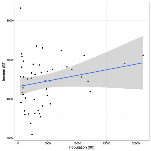
We also went over using R Markdown files to interweave R code and text for use
when you make a manuscript or thesis! See the example here.
To convert this file to a Word document, you can type Ctrl-Shift-K (for knit).
Resources
- Official R website with a list of packages
- Learning R for data analysis (excellent resource!)
- Rstudio cheatsheets (also
found in
Help -> Cheatsheetsin Rstudio)